full-length paper  — code available upon request

Abstract

The newsvendor model is a mathematical problem that has appeared in several mathematical journals for use cases ranging from determining cash reserves to selling Christmas trees ¹. The model is used to determine the optimal inventory level. It is referred to as the “newsvendor problem” because newsvendors needed to purchase large quantities of newspapers to sell but faced uncertain demand.

Some days demand could be high or low, and the vendor is stuck with any leftover newspapers, this is why calculating the optimal order quantity is important. An optimal order quantity is returned by the model ¹, and Monte Carlo simulations then show the newsvendor the profit they can expect when using that optimal order quantity

Background

The classic newsvendor problem determines the optimal order quantity given stochastic demand. Previously it has been applied to credit applications, reservations, return policies, and many other fields. Recently, blockchain technology’s impact on the newsvendor problem has been studied. Chang et al. (2021) concluded that by embedding blockchain adoption into the newsvendor model, it is possible to “boost the demand size” and “reduce demand uncertainty” ².

The web application I developed aims to bring the Monte Carlo simulation method to the newsvendor problem in an interactive application. The goal of this application is to provide a way for vendors to easily determine and visualize potential profits.

Assumptions of the newsvendor model

The newsvendor model is based on the following assumptions:

• The demand is random and follows a known probability distribution
• The selling price, cost, and salvage value of the product are known and fixed
• Buying decisions are made before the actual demand is known¹

Critical Fractile

The critical fractile ratio is determined by the following formula, where $p$ is the unit selling price, $c$ is the unit cost, and $s$ is the salvage price for unsold inventory:

$$g = \frac{p - c}{p - s}$$

$g$ represents the probability that demand exceeds the chosen order quantity. If this ratio is greater than $\tfrac{1}{2}$, it is defined as a high‑profit ³. This ratio helps determine both the chance that demand will exceed the order quantity and the value of the optimal order quantity.

Optimal Order Quantity

As shown by Porteus ¹, the optimal order quantity $Q^*$ for a normally distributed demand is:

$$Q^* = \mu + z^*(g)\,\sigma$$

where $\mu$ and $\sigma$ are the mean and standard deviation of demand, and $z^*(g)$ is the inverse cumulative distribution function evaluated for the critical fractile $g$. In this project, the simulation uses $Q^*$ for each run as the ordered quantity, allowing us to see the theoretical performance of thousands of simulated demand realizations.

My Approach

The application is designed to be a user-friendly Python web application that allows the end users to input parameters such as price, cost, salvage value, demand, etc. and see how the model performs based on thousands of simulated demands.

First, the inputs are used to generate the optimal order quantity and critical fractile. Then simulations are run and for each simulation, a random demand is generated based on the mean, distribution, and standard deviation entered by the user. Using the price, cost, and salvage price of the units, the application checks to see if the seller would have run out of inventory (stock out) or if the seller would have profited and how much they would have earned for each run. Finally, visualizations are generated to show the cumulative average profit and the histogram of the demand and profit distributions.

Development

Inputs

There are three types of inputs: demand characteristics, financial parameters, and the simulation settings.

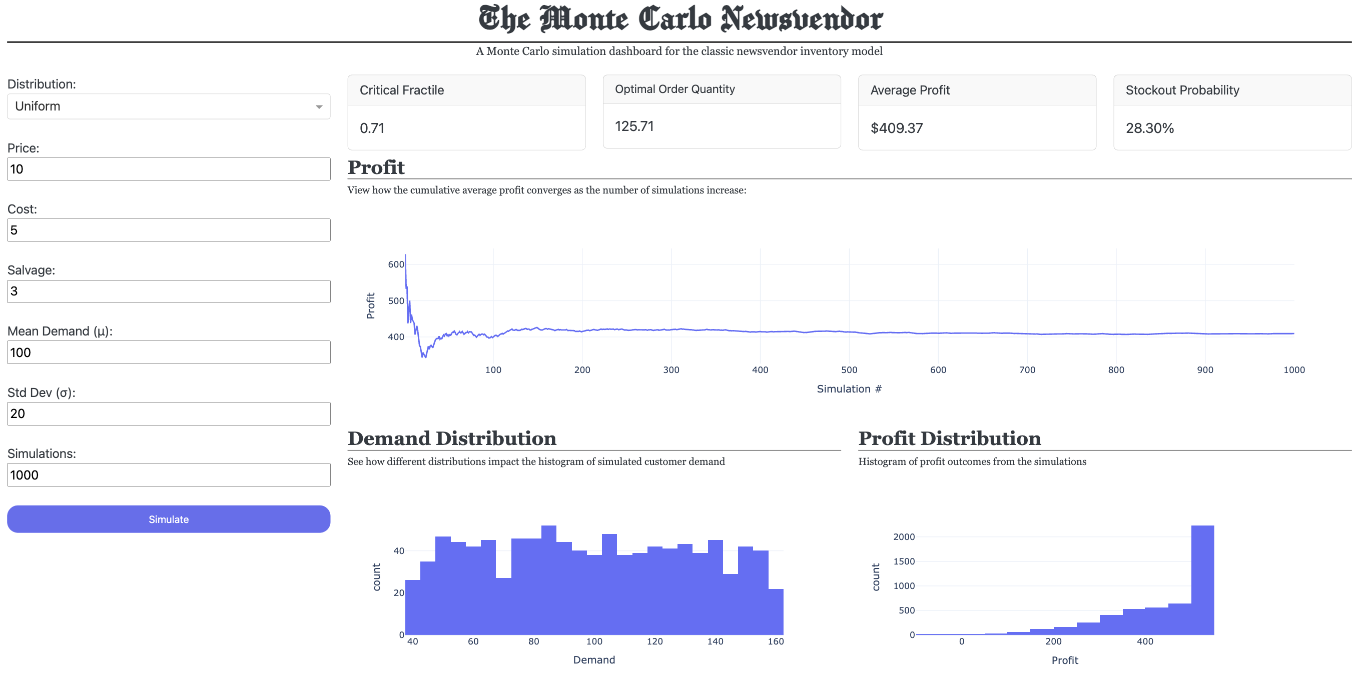
The program allows the user to input one of three demand distributions in a single-select dropdown. The distributions are normal, uniform, and exponential. For any of the demand distributions, the mean and standard deviation are entered as a text field. For the financial parameters, there are text fields to input the price, cost, and salvage. Finally, the number of simulations is entered using a text field. After all seven inputs are filled, or by using the default inputs, the user presses the button labeled “Simulate”, and the app will run.

Figure 1: Inputs for the Monte Carlo Newsvendor application

Outputs

The profit visualization displays the cumulative average profit over all simulations. This allows the end-user to visually see how many simulations it will take for the average profit to reach a consistent level.

Figure 2: Cumulative Profit Chart

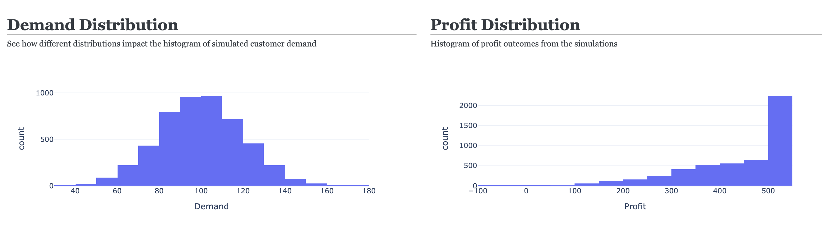
The two charts on the bottom of the dashboard (Figure 3) indicate two distributions, one for demand and one for profit. The demand distribution is a histogram of the randomly generated demand of each simulation. The profit distribution is a histogram of the profit that was calculated for each simulation.

Figure 3: Histograms

Architecture

The Monte Carlo Newsvendor application consists of four core functions, HTML, and Plotly Dash components to build the web application. The 4 core functions are listed below:

• critical_fractile()
• optimal_order_quantity()
• get_random_demand()
• simulation()

critical_fractile() and optimal_order_quantity()

At the core of all newsvendor models (including my application) are two formulas: critical_fractile and optimal_order_quantity. The critical_fractile function takes price $p$, cost $c$, and salvage price $s$ as inputs and returns the critical fractile $g$. The optimal_order_quantity function computes the order quantity that balances the risk of stockouts against excess inventory requiring salvage. It calls critical_fractile to obtain f_star, and then, based on the specified distribution, uses SciPy’s percent-point function (the inverse CDF is called using .ppf) to calculate the optimal order quantity ⁴.

get_random_demand()

In order to implement Monte Carlo simulation, this application generates a random demand for each simulation using the get_random_demand function. The simplest way to do this was by invoking NumPy’s random number generator⁵. The advantage of using this package’s built-in function is that it can easily adapt to different distributions.

simulation()

The most important function in my entire application is the simulation function. It’s parameters include all the inputs and the optimal order quantity. This function handles going through each simulation, processing its inputs and returning statistics which are used in the output displays. For each run of the simulation a random demand is generated, and since we are using the same order quantity each time, this function then calculates sales, revenue, profit, and stockouts. Sales are calculated by finding the minimum of the demand and optimal order quantity, whichever is smaller is the amount sold for that period. Finally, the profit and stockouts are calculated as averages and used to update the dashboard.

HTML, Dash, Bootstrap, and Callback

Prior to this project, I did not have much experience building web applications, including Plotly Dash apps. However, using Plotly’s online resources made it easy to build my application from HTML divs and Dash’s core components for the rows and columns. I did further research to build and place graphs and charts using Plotly. Then implemented Dash’s Bootstrap themes to style the application and make it visually appealing. The final element of my code is the callback and update simulation function. This part of the code houses the core functions I described and updates the visuals by using a callback function. The callback function is triggered when the user presses the “Simulate” button.

Figure 4: Full Dashboard

Conclusion and Future Implementations

One of my major takeaways from developing and using this application was that you can clearly see the impacts of different profit margins and salvage prices. If you can keep a low cost and maintain a salvage price close to the cost, it will lead to a much higher profit. The reason for this being that there is much less risk and order quantity can go much higher which also leads to a lower risk of stockouts.

One thing that could be improved upon using my application is utilizing real-world data. An article from the European Journal of Operational Research states that “in reality, the true demand distribution is hardly ever known to the decision maker”⁶. Their study showed that data-driven demand and inventory optimization could “outperform their model-based counterparts”⁶. If I were to continue with this project, I would like to give users an option to allow for uploading real demand data because. This feature would allow vendors to see realistic performance metrics and allow for experimentation that could positively impact their business.

---

Footnotes

1. Porteus, E. L. (2008). The Newsvendor Problem. In D. Chhajed & T. J. Lowe (Eds.), Building Intuition (Vol. 115, pp. 193–213). Springer, Boston, MA. https://doi.org/10.1007/978-0-387-73699-0_7  ↩ ↩² ↩³ ↩⁴

2. Chang, J., Katehakis, M. N., Shi, J., & Yan, Z. (2021). Blockchain‑empowered Newsvendor optimization. International Journal of Production Economics, 238, 108144. https://doi.org/10.1016/j.ijpe.2021.108144  ↩

3. Schweitzer, M. E., & Cachon, G. P. (2000). Decision Bias in the Newsvendor Problem with a Known Demand Distribution: Experimental Evidence. Management Science, 46(3), 404–420. https://doi.org/10.1287/mnsc.46.3.404.12070  ↩

4. SciPy (2025). Percent point function (inverse CDF). Retrieved April 5, 2025, from https://docs.scipy.org/doc/scipy/reference/generated/scipy.stats.rv_continuous.ppf.html  ↩

5. NumPy (2025). Random module reference. Retrieved April 5, 2025, from https://numpy.org/doc/2.1/reference/random/index.html  ↩

6. Huber, J., Müller, S., Fleischmann, M., & Stuckenschmidt, H. (2019). A data‑driven newsvendor problem: From data to decision. European Journal of Operational Research, 278(3), 904–915. https://doi.org/10.1016/j.ejor.2019.04.043  ↩ ↩²